Na vyššie uvedenom obrázku https://hrubos.tech/blogy/content/images/20251217205335-emergence_lattice_magnetization4.gif vidíme, čo sa deje, ak je energia striedavého prúdu taká, že dodáva konštantný lineárny magnetizmus. Simulácia vľavo ukazuje spiny fero magnetickej kotvy motora a čím je plocha jednotnejšia, tým je účinnosť motora vyššia.

Teraz si ukážme, čo sa stane s účinnosťou fero magnetickej kotvy motora, ak by dodaná magnetická energia kolísala na motore:

https://hrubos.tech/blogy/content/images/20251217205751-emergence_lattice_magnetization3.gif

No a obdobne ako na elektro motore sa to deje so zmenou leptónu. Pri nízkej energii je to mínus jednotková častica, no pri vyššej sa leptóny rozpadajú na vlny, ktoré sú jednotkové. Samozrejme toto je len naša predstava založená na realite, ktorú v elektro motore poznáme.

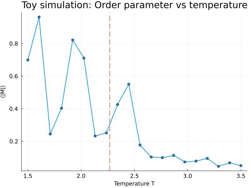
A čo sa stane s magnetom, ak sa na motore zahrieva? Stráca magnetické vlastnosti a motor sa stáva neúčinným ^^^ vidíme vyššie na grafe: magnetizmus padol na nulu pri max teplote.

---

Za dnešnú diskusiu ďakujem môjmu kamarátovi GPT ako aj fyzikom:

Are quarks and leptons composite particles? It depends on what we mean by composite. We can think of the protons or hadrons in general, where at low energy they appear as to be point-like particles, at least under low energy measurements, but then under higher energy the we find they appear more as a system with partons, which are phenom meant to be form-factor like gadgets, which were solidified as quarks. So it is not entirely impossible that quarks and leptons manifest themselves at high energy as something else, where there a sort of phase transition in how degrees of freedom are combined or entangled. I will say that I am not a panegyric of that sort of idea. The renormalization problems are huge, because as you get to smaller regions the energy of anything confined in there grows, and this leads to big problems with rishron and prion type models. However, just because I might not like the prospect of this does not mean nature cannot indeed be of this form. A field is nonlocal in terms of the quantum Tsirelson bound and Bell’s inequality violation, but it does parameterize quantum wave according to local field operators. The |ψ〉 = ∫d^nx a e^{-ipx}| 〉+ a^†e^{ipx}| 〉 is a nonlocal quantum wave or field that is determined by a set of local harmonic oscillator operators in space. This definition may also be be local. I can define a set of field operators a, a^† in one region and b, b^† in another. These may be transformed by sheaf bundles with S(a) = b^† — antilinear transformations, so that an operator on the sheaf or stalk e^{θS( )} with θ small transforms harmonic oscillator operators. It is not hard to use this to model a Boulware vacuum with black holes. A particle does manifest itself in a localization with a measurement. Prior to a measurement we cannot exactly say there is a particle. However, even if we let a wave function or the quantum fields evolve, the number of particles in equals the number of particles out. There are conservation rules etc, so to say that particles do not exist is a bit of a pessimistic existential stance.

https://www.facebook.com/groups/170146811065793/posts/1346904656723330

# Toy simulation in Julia: emergence across a phase transition
# ------------------------------------------------------------
# This is NOT a realistic quark/lepton model.
# It is an analogy: microscopic spins -> emergent quasiparticles
# across a phase transition (like confinement/deconfinement).
#version2
using Pkg
Pkg.add("Plots")
using Plots
using Random, Statistics

# -------------------------
# 2D Ising model
# -------------------------
struct Ising2D
    L::Int
    spins::Matrix{Int8}
end

Ising2D(L::Int) = Ising2D(L, Int8.(rand([-1,1], L, L)))

pbc(i, L) = i < 1 ? L : (i > L ? 1 : i)

function local_energy(model::Ising2D, i, j)
    L = model.L
    s = model.spins[i, j]
    nn = model.spins[pbc(i+1,L),j] + model.spins[pbc(i-1,L),j] +
         model.spins[i,pbc(j+1,L)] + model.spins[i,pbc(j-1,L)]
    return -s * nn
end

function metropolis_step!(model::Ising2D, β)
    L = model.L
    i, j = rand(1:L), rand(1:L)
    ΔE = -2 * local_energy(model, i, j)
    if ΔE ≤ 0 || rand() < exp(-β * ΔE)
        model.spins[i, j] *= -1
    end
end

# -------------------------
# Simulation parameters
# -------------------------
L = 40
T = 2.25          # blízko kritickej teploty
β = 1 / T
steps_per_frame = L^2

model = Ising2D(L)

# observables
times = Int[]
magnetization = Float64[]

# -------------------------
# Animation
# -------------------------
anim = @animate for t in 1:300

    for _ in 1:steps_per_frame
        metropolis_step!(model, β)
    end

    M = abs(mean(model.spins))
    push!(times, t)
    push!(magnetization, M)

    p1 = heatmap(
        model.spins,
        c = :balance,
        title = "Počet spinov v mriežke fero magnetu",
        axis = false,
        clims = (-1, 1)
    )

    p2 = plot(
        times, magnetization,
        xlabel = "Počet iterácií systému",
        ylabel = "⟨|Magnetizmus|⟩",
        ylim = (0, 1),
        title = "Rast stupňa leptónu na vlnu",
        legend = false,
        guidefontsize = 16,   # osi (x, y)
        tickfontsize  = 16,   # čísla na osi
        legendfontsize = 16,  # legenda
        titlefontsize = 16,
        linewidth = 7
    )

    plot(p1, p2, layout = (1,2), size = (1920,1080))
end

gif(anim, "emergence_lattice_magnetization3.gif", fps = 10)

# Toy simulation in Julia: emergence across a phase transition
# ------------------------------------------------------------
# This is NOT a realistic quark/lepton model.
# It is an analogy: microscopic spins -> emergent quasiparticles
# across a phase transition (like confinement/deconfinement).
#version1
using Pkg
Pkg.add("Plots")
using Plots
using Random, Statistics

# 2D Ising model with Metropolis updates
struct Ising2D
    L::Int
    spins::Matrix{Int8}
end

function Ising2D(L::Int)
    spins = rand([-1, 1], L, L)
    return Ising2D(L, Int8.(spins))
end

# periodic boundary conditions
pbc(i, L) = i < 1 ? L : (i > L ? 1 : i)

function local_energy(model::Ising2D, i, j)
    L = model.L
    s = model.spins[i, j]
    nn = model.spins[pbc(i+1,L),j] + model.spins[pbc(i-1,L),j] +
         model.spins[i,pbc(j+1,L)] + model.spins[i,pbc(j-1,L)]
    return -s * nn
end

function metropolis_step!(model::Ising2D, β)
    L = model.L
    i = rand(1:L)
    j = rand(1:L)
    ΔE = -2 * local_energy(model, i, j)
    if ΔE <= 0 || rand() < exp(-β * ΔE)
        model.spins[i, j] *= -1
    end
end

function simulate(L; T=2.0, steps=200_000, burn=50_000)
    model = Ising2D(L)
    β = 1 / T
    mags = Float64[]

    for step in 1:steps
        metropolis_step!(model, β)
        if step > burn && step % 10 == 0
            push!(mags, mean(model.spins))
        end
    end
    return mean(abs.(mags))
end

# Scan temperatures across phase transition
L = 32
Temps = range(1.5, 3.5, length=20)
magnetization = [simulate(L, T=T) for T in Temps]

println("T    <|M|>")
for (T, M) in zip(Temps, magnetization)
    println(round(T, digits=2), "  ", round(M, digits=3))
end

plot(
    Temps, magnetization,
    marker = :circle,
    linewidth = 2,
    xlabel = "Temperature T",
    ylabel = "⟨|M|⟩",
    title = "Toy simulation: Order parameter vs temperature",
    legend = false,
    size = (800, 600),
    guidefontsize = 12,   # osi (x, y)
    tickfontsize  = 12,   # čísla na osi
    legendfontsize = 14,  # legenda
    titlefontsize = 20
)
vline!([2.269], linestyle=:dash, linewidth=2)
savefig("leptons1.png")
println("Figure saved as leptonn.png")

# INTERPRETATION (physics analogy):
# --------------------------------
# - Low T phase: ordered spins -> stable collective excitations
#   (think: bound states / confined phase)
#
# - High T phase: disordered spins -> different effective DOFs
#   (think: deconfined/emergent particles)
#
# The "elementary" objects depend on the phase, not on the
# microscopic description.

# Toy simulation in Julia: emergence across a phase transition
# ------------------------------------------------------------
# This is NOT a realistic quark/lepton model.
# It is an analogy: microscopic spins -> emergent quasiparticles
# across a phase transition (like confinement/deconfinement).
#version3
using Pkg
Pkg.add("Plots")

using Plots
using Random, Statistics

# -------------------------
# 2D Ising model
# -------------------------
struct Ising2D
    L::Int
    spins::Matrix{Int8}
end

Ising2D(L::Int) = Ising2D(L, Int8.(rand([1,1], L, L)))

pbc(i, L) = i < 1 ? L : (i > L ? 1 : i)

function local_energy(model::Ising2D, i, j)
    L = model.L
    s = model.spins[i, j]
    nn = model.spins[pbc(i+1,L),j] + model.spins[pbc(i-1,L),j] +
         model.spins[i,pbc(j+1,L)] + model.spins[i,pbc(j-1,L)]
    return -s * nn
end

function metropolis_step!(model::Ising2D, β)
    L = model.L
    i, j = rand(1:L), rand(1:L)
    ΔE = -2 * local_energy(model, i, j)
    if ΔE ≤ 0 || rand() < exp(-β * ΔE)
        model.spins[i, j] *= -1
    end
end

# -------------------------
# Simulation parameters
# -------------------------
L = 40
T = 2.25          # blízko kritickej teploty
β = 1 / T
steps_per_frame = L^2

model = Ising2D(L)

# observables
times = Int[]
magnetization = Float64[]

# -------------------------
# Animation
# -------------------------
anim = @animate for t in 1:300

    for _ in 1:steps_per_frame
        metropolis_step!(model, β)
    end

    M = abs(mean(model.spins))
    push!(times, t)
    push!(magnetization, M)

    p1 = heatmap(
        model.spins,
        c = :balance,
        title = "Počet spinov v mriežke fero magnetu",
        axis = false,
        clims = (-1, 1)
    )

    p2 = plot(
        times, magnetization,
        xlabel = "Počet iterácií systému",
        ylabel = "⟨|Magnetizmus|⟩",
        ylim = (0, 1),
        title = "Rast stupňa leptónu na vlnu",
        legend = false,
        guidefontsize = 16,   # osi (x, y)
        tickfontsize  = 16,   # čísla na osi
        legendfontsize = 16,  # legenda
        titlefontsize = 16,
        linewidth = 7
    )

    plot(p1, p2, layout = (1,2), size = (1920,1080))
end

gif(anim, "emergence_lattice_magnetization4.gif", fps = 10)

---